import pandas as pd
from ucimlrepo import fetch_ucirepo
from sklearn.model_selection import train_test_split
from tabicl import TabICLRegressor

wine = fetch_ucirepo(id=186)
X = wine.data.features
y = wine.data.targets["quality"]

X_train, X_test, y_train, y_test = train_test_split(
    X, y, test_size=0.25, random_state=1
)7 Regression
Tabular foundation models predict continuous targets the same way they classify, through in-context learning. Their predictions are an ensemble, which makes speed and accuracy directly tradeable.
You can use tabular foundation models like TabICL also for regression. The regression foundation models are based on different pretraining, and a slightly different architecture, but otherwise, feel and look are very similar to classification.
Let’s use TabICL to make predictions.
Let’s predict wine quality
We will predict the quality of wines based on their physical and chemical properties like alcohol content and acidity. We use the Wine Quality dataset (Cortez et al. 2009) from the UCI Machine Learning Repository, which collects red and white vinho verde samples from northern Portugal.
Let’s load the dataset and create a train-test split.
print(X_train.head().T.to_markdown())| 275 | 3406 | 3163 | 4623 | 2527 | |
|---|---|---|---|---|---|
| fixed_acidity | 7.9 | 8.8 | 9.1 | 7 | 6.5 |
| volatile_acidity | 0.545 | 0.2 | 0.28 | 0.13 | 0.25 |
| citric_acid | 0.06 | 0.43 | 0.49 | 0.37 | 0.35 |
| residual_sugar | 4 | 15 | 2 | 12.85 | 12 |
| chlorides | 0.087 | 0.053 | 0.059 | 0.042 | 0.055 |
| free_sulfur_dioxide | 27 | 60 | 10 | 36 | 47 |
| total_sulfur_dioxide | 61 | 184 | 112 | 105 | 179 |
| density | 0.9965 | 1.0008 | 0.9958 | 0.99581 | 0.998 |
| pH | 3.36 | 3.28 | 3.15 | 3.05 | 3.58 |
| sulphates | 0.67 | 0.79 | 0.46 | 0.55 | 0.47 |
| alcohol | 10.7 | 8.8 | 10.1 | 10.7 | 10 |
Predict in-context with TabICL
Let’s predict the wine quality data with the in-context learning capabilities of TabICL.
reg = TabICLRegressor(random_state=1)
reg.fit(X_train, y_train)

y_pred_tabicl = reg.predict(X_test)
y_pred_tabicl[:5].round(2)
array([5.35, 5.02, 5.29, 5.65, 5.07], dtype=float32)By default, TabICL predicts the mean of the predictive distribution. TabICL makes it super easy to instead predict the median by simply changing one parameter:
y_pred_median = reg.predict(X_test, output_type="median")
y_pred_median[:5].round(2)
array([5. , 5. , 5.01, 5.99, 4.99], dtype=float32)But again, thanks to the scikit-learn interface, TabICL usage feels very similar to traditional machine learning, even though we don’t train the model with fit, and predict does in-context learning.
Let’s evaluate the model, and also compare it with a CatBoost tree ensemble.
TabICL versus CatBoost
To compare TabICL against CatBoost (Prokhorenkova et al. 2018), let’s tune CatBoost’s most commonly tuned hyperparameters with random search:
from catboost import CatBoostRegressor
from scipy.stats import loguniform, randint, uniform
from sklearn.model_selection import RandomizedSearchCV

param_distributions = {
    "learning_rate":       loguniform(1e-2, 3e-1),
    "depth":               randint(4, 11),
    "l2_leaf_reg":         loguniform(1.0, 10.0),
    "bagging_temperature": uniform(0.0, 1.0),
}

cat_search = RandomizedSearchCV(
    CatBoostRegressor(iterations=500, random_state=1, verbose=False, thread_count=1),
    param_distributions,
    n_iter=40,
    scoring="neg_root_mean_squared_error",
    random_state=1,
    n_jobs=-1,
)
cat_search.fit(X_train, y_train)

y_pred_cat = cat_search.predict(X_test)
And the comparison:
from sklearn.metrics import mean_absolute_error, mean_squared_error, r2_score

def regression_score(y_true, y_pred):
    return {
        "MAE":  mean_absolute_error(y_true, y_pred),
        "RMSE": mean_squared_error(y_true, y_pred) ** 0.5,
        "R²":   r2_score(y_true, y_pred),
    }

print(pd.DataFrame({
    "TabICL":         regression_score(y_test, y_pred_tabicl),
    "Tuned CatBoost": regression_score(y_test, y_pred_cat),
}).round(3).to_markdown())| TabICL | Tuned CatBoost | |
|---|---|---|
| MAE | 0.388 | 0.435 |
| RMSE | 0.577 | 0.602 |
| R² | 0.546 | 0.507 |
In all three metrics, TabICL beats the CatBoost ensemble. This is of course not guaranteed to happen, but benchmarks have shown that TFMs often best boosted tree ensembles, the previously strongest models in the tabular space. But did you know that our TabICL regressor is an ensemble, too?
TabICL is an ensemble
When calling reg.predict, the function actually returns an average prediction across an ensemble of 8 TabICL predictions for each row.
That might be a quite puzzling fact at first: How do the predictions differ, and what is the motivation for ensembling predictions of TFMs? Ensembling is typically used to improve predictive performance, and make predictions more robust. Performance and robustness are also the motivation behind TabICL ensembling.
A good ensemble is built on variety: it benefits from diversity of the underlying ensemble members, aka machine learning models. So, where is the variety coming from between two different TabICL models in this ensemble? There are a couple of knobs that can be randomized to create prediction diversity (three for classification):
- The order of the features, which may be re-arranged by circular shifts, random permutation, Latin square, or kept as-is.
- The feature pre-processing transformation used. Default is to pick between the Yeo-Johnson power transformation (Yeo and Johnson 2000), and no transformation.
- For classification, the order of the class labels may be randomized.
But why does shuffling the features create diversity? Sounds … bad. And, indeed, it’s an artifact of an architectural choice of TabICL and other TFMs. The attention mechanism can’t distinguish features that have the same marginal distribution (i.e. same means, same variance, …), and to counteract that, features are grouped within the architecture. But that also means that the predictions depend on the order of features. That also makes ensembling more than just a fun option: conceptually, there is no “right” order of features, so it makes sense to smooth that out by averaging over various feature orders.
Trading accuracy for speed with n_estimators
By default, the prediction is averaged over doing 8x TabICL in-context learning with different pre-processing and feature orders (and class label order, in case of classification). Since prediction is the expensive step with TFMs, this also means reducing ensemble size is a huge cost lever. A lever that can reduce prediction time by a factor of roughly 8.
Try reducing
n_estimators
With the default being 8 estimators, there is an up to 8x inference speed improvement. It’s always worth trying out using fewer estimators in the ensemble.
But this comes at a price: Reducing ensemble sizes sometimes reduces predictive performance and robustness. Since this may differ between tasks and applications, it’s always worth trying out. Let’s see whether and how the performance suffers and prediction time improves when we reduce the ensemble size for the wine quality prediction.
from time import perf_counter

results = []
for n in [1, 2, 4, 8]:
    reg = TabICLRegressor(n_estimators=n, random_state=1)
    reg.fit(X_train, y_train)

    start = perf_counter()
    pred = reg.predict(X_test)
    elapsed = perf_counter() - start

    results.append({
        "n_estimators": n,
        "predict (s)":  elapsed,
        **regression_score(y_test, pred),
    })

df = pd.DataFrame(results).set_index("n_estimators")
print(df.round(3).to_markdown())| n_estimators | predict (s) | MAE | RMSE | R² |
|---|---|---|---|---|
| 1 | 5.327 | 0.39 | 0.58 | 0.542 |
| 2 | 8.751 | 0.388 | 0.578 | 0.545 |
| 4 | 17.932 | 0.388 | 0.578 | 0.545 |
| 8 | 51.986 | 0.388 | 0.577 | 0.546 |
import matplotlib.pyplot as plt

fig, ax = plt.subplots(figsize=(6.5, 4))
ax2 = ax.twinx()
ax.plot(df.index, df["predict (s)"], "o-", color="#3b6ea5")
ax2.plot(df.index, df["R²"], "s-", color="#c0392b")
ax.set(xlabel="Ensemble size (`n_estimators`)", ylabel="predict time (s)",
       xticks=df.index, ylim=(0, None))
ax2.set(ylabel="R²", ylim=(0, 1))
for x, y in zip(df.index, df["R²"]):
    ax2.annotate(f"{y:.3f}", (x, y), xytext=(0, -10), textcoords="offset points",
                 ha="center", va="top", color="#c0392b", fontsize=9)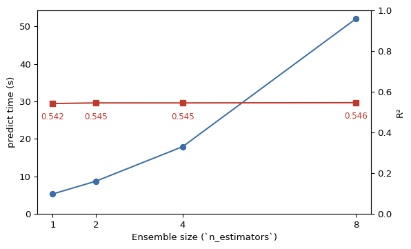
For the wine data, it seems that actually having just one TabICL in-context pass is enough, no need for a varied ensemble. And an easy way to reduce compute time by roughly 87.5%!