2  Prior-data fitted networks

By the end of this chapter, you’ll:

• get an idea of prior-data fitted networks (PFNs), the base for foundation models such as TabPFN.
• (optional) understand the Bayesian motivation for PFNs: approximating the posterior predictive distribution by sampling tasks from a prior.

There is a difference between “traditional” machine learning and foundation models:

• Models such as boosted tree ensembles must be trained from scratch each time.
• Foundation models like TabPFN are pretrained on millions of datasets and predict via in-context learning.

Definition: In-Context Learning

When a model dynamically adapts to a task without optimizing any parameters.

In this chapter, we take a look at the fundamental idea that makes models like TabPFN and TabICL foundation models.

Tables are messy

Data modalities like image and text have had foundation models already before tabular. For example, the Generative Pretrained Transformers (GPT) (Radford et al. 2018), the base for most large language models, is pretrained to predict tokens, which then can be leveraged to do other things like translation. One of the reasons for tabular to be such a late bloomer: tables are messy. I mean, compare it to images: they can be squeezed into the same rectangular shape and each feature has the same interpretation: it’s a pixel. If image data is like a box full of photos, tabular is your junk drawer full of half-empty batteries, mysterious screws, and cables you no longer need:

• One table has 3 columns, another has 30,000.
• One column is named “sales_fruit_banana”, the other is “id_12319_ban”, both contain the same data.
• Just kidding. “sales_fruit_banana” contains the store’s total monthly sales of bananas; “id_12319_ban” contains only sales for brand “MonkeyNeverCramp”. Only Bob from marketing knows this.
• Two columns contain numbers from 1-10. For one column, these are counts, for the other, categories.
• If you shuffle the rows or columns of a dataset, it’s conceptually the same dataset.
• There are missing values everywhere.

For these reasons, I’m still mad at the first person to call tables “structured” data. Even if you have two tables capturing similar information, they may differ in myriads of ways. That made it challenging to come up with an algorithm that can learn generalizable patterns from tables that can be transferred to other tables. Fortunately, in 2022, an approach called prior-data fitted networks emerged, that would become the basis of an entire family of tabular foundation models.

PFNs combine pretraining and in-context learning

Tabular foundation models such as TabPFN and TabICL are based on an approach called prior-data fitted networks (PFNs) (Müller et al. 2022).¹ PFNs are a more general framework of how to infuse prior knowledge into a model, such as mimicking Gaussian processes or few-shot image-classification. The most prominent application of PFNs, by far, is tabular foundation models.

The core idea behind PFNs: Pretrain a model on a prior collection of tasks so that it can later perform in-context learning of the target distribution.

Definition: Task

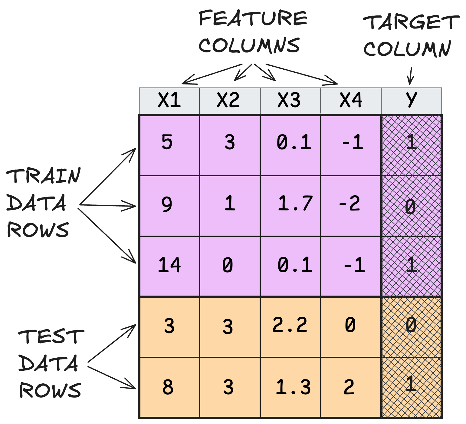
A task is defined by

• table +
• train-test indicator +
• target-feature indicator.

Or, equivalently, a task is:

• training feature matrix +
• training target matrix +
• test feature matrix
• test target matrix (optional).

An ML task also has an objective \(L\), but it’s the same for every task in the prior.

PFNs “solve” foundation models by moving everything up one level of abstraction, compared to traditional machine learning. In traditional machine learning, we have one dataset on which we train a model, and then predict using the trained model. PFN-based foundation models move away from this train-then-predict paradigm to pretrain-then-ICL:

• Instead of training on a single dataset, TFMs are pretrained on millions of datasets.
• For traditional machine learning, a dataset row is the fundamental unit they operate on. For PFN-based learning, it’s entire datasets, or rather, supervised ML tasks.
• Instead of prediction which accepts individual rows, TFMs do in-context learning, requiring the entire table of training and new data.

To allow for this paradigm change, a few ingredients are involved:

• A model with a flexible architecture: We need a flexible architecture, that accepts an entire dataset as one “data point”, so that it can do in-context learning with an entire task and be pretrained with batches of datasets. This architecture is typically a transformer-based neural network with row- and column-attention mechanisms. Once pretrained, this model can then do in-context learning. Meaning we can shove an entire table through, get predictions without needing to change any weights.
• A prior from which we can sample tasks: To pretrain a model like TabPFN, we need millions of tasks. These are typically synthetic, that is, they are generated by a procedure, also called the prior. Structural causal models have emerged as a key method for the prior.
• A pretraining procedure: During pretraining, batches of tasks are generated on the fly from the prior distribution. Using gradient-descent, the tabular foundation model is trained to predict the predictive distribution of the test target. The loss used is typically the negative log likelihood across the prior.

PFNs have a Bayesian interpretation

At inference time, PFN-based tabular foundation models approximate the posterior prediction distribution of the test target conditional on test features and training data. The task prior is therefore really a prior in the Bayesian sense.

Mathematical motivation for PFNs

The goal is to model the posterior predictive distribution:

\[ p(y|x_{new}, X_{train}, y_{train}) \]

To allow for prior knowledge we blow up this term with the law of total probability, with latent variable \(\phi\) representing the underlying supervised ML tasks.

\[ p(y|x_{new}, X_{train}, y_{train}) = \int_{\phi} p(y|x_{new},\phi) p(\phi|X_{train}, y_{train})d\phi \]

We can’t really handle \(p(\phi|X_{train}, y_{train})\), so we apply Bayes’ theorem to flip it into terms we can sample from:

\[ p(y|x_{new}, X_{train}, y_{train}) = \int_{\phi} p(y|x_{new},\phi) \, \frac{p(X_{train}, y_{train}|\phi)\, p(\phi)}{p(X_{train}, y_{train})} \, d\phi \]

The denominator \(p(X_{train}, y_{train})\) does not depend on \(\phi\), so it’s a constant factor. Dropping it, we can write the posterior predictive distribution, up to that constant, as:

\[ \underbrace{\bbox[#E8ECEF,3px,border:1px solid #7A7F85]{p(y \mid x_{\text{new}}, X_{\text{train}}, y_{\text{train}})}}_{\substack{\text{posterior predictive}\\\text{distribution}}} \;\propto\; \underbrace{ \bbox[#A3D8FF,3px,border:1px solid #2E7BC0]{\int_\phi}\, \overbrace{\bbox[#B3F2BB,3px,border:1px solid #2E9440]{p(y \mid x_{\text{new}}, \phi)}}^{{\color{#2E9440}\substack{\text{task-conditional}\\\text{predictive distribution}}}} \overbrace{\bbox[#FFCED2,3px,border:1px solid #D83A3A]{p(X_{\text{train}}, y_{\text{train}} \mid \phi)}}^{{\color{#D03030}\substack{\text{data likelihood}\\\text{conditional on task}}}} \overbrace{\bbox[#FFE6A5,3px,border:1px solid #E69100]{p(\phi)}}^{{\color{#E08000}\substack{\text{prior}\\\text{over tasks}}}}\, \bbox[#A3D8FF,3px,border:1px solid #2E7BC0]{d\phi} }_{{\color{#1070C0}\text{integrate over supervised ML tasks}}} \]

In the next chapter, we take a deeper look at in-context learning.

Müller, Samuel, Noah Hollmann, Sebastian Pineda Arango, Josif Grabocka, and Frank Hutter. 2022. “Transformers Can Do Bayesian Inference.” In International Conference on Learning Representations (ICLR). https://doi.org/10.48550/arXiv.2112.10510.

Radford, Alec, Karthik Narasimhan, Tim Salimans, and Ilya Sutskever. 2018. “Improving Language Understanding by Generative Pre-Training.” OpenAI. https://cdn.openai.com/research-covers/language-unsupervised/language_understanding_paper.pdf.

---

1. Prior-data fitted networks (PFNs) is also what gave TabPFN its name.