3 In-context learning
- Explain why tabular foundation models keep and use training data at prediction time.
- Understand how table cells become vectors that get progressively enriched by attention to other cells and individual refinement.
Let’s get a first idea of how tabular foundation models (TFMs) make predictions. For the sake of this chapter, assume that the tabular foundation model is already pretrained. Since TFMs are large neural networks, this means their weights are all set, and we can apply them to data to make predictions.
This chapter focuses on how the data is represented and reshaped as it travels through the TFM, and less on the architecture. Just like it’s useful to understand that clay is burned to make a cup, before explaining how the oven works.
Actual implementations of most TFMs are more complex than described here. The TFM that comes closest is nanoTabPFN (Pfefferle et al. 2025), an educational implementation of TabPFN v2.
TFMs do in-context learning
In traditional machine learning, we start out with a dataset and split it into training and test data, at least in the simplest version (see Figure 3.1). We use the training data to train the model, and evaluate it on the test data. Thereby, the ML algorithm learns a model that predicts the target column(s) from the feature columns. To make predictions, the model then needs the feature columns for the new data.
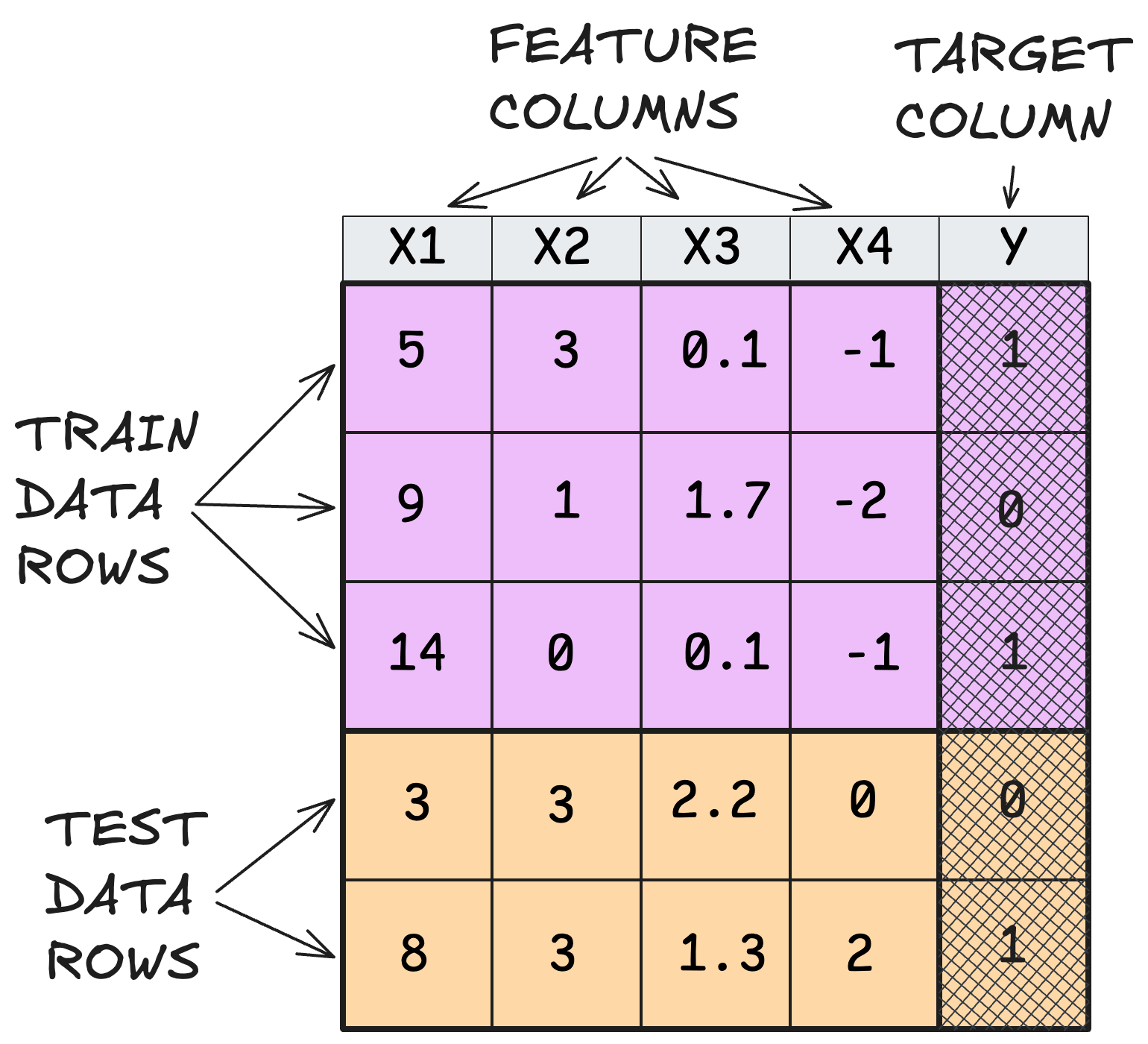
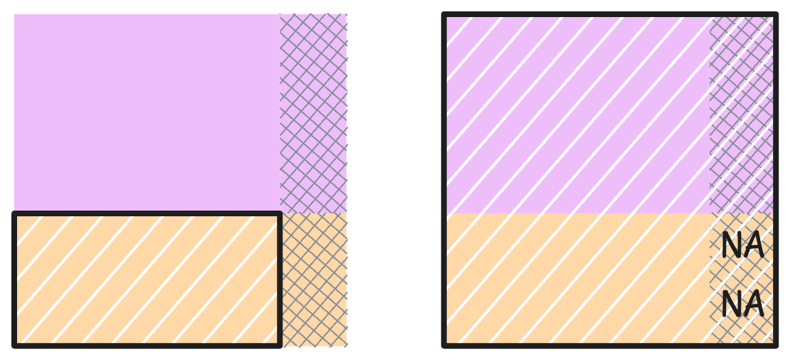
So far, so good, I hope the previous paragraph was boring to you. For TFMs, the predict step works quite differently: besides the test features1, it also needs the training data at prediction time. Actually, it also needs the test targets, but pre-filled with missing values or mean imputation from the training data. Otherwise it would be cheating of the highest order, punishable by exile to Excel. Figure 3.2 visualizes this shift of predict-input when moving from traditional to foundational modeling.
Hold on a second! In Chapter 1, the very first TFM code example was: clf.fit(X_train, y_train) and then clf.predict(X_test), suggesting a traditional train-test split. However, we must distinguish between the programming interface and the underlying objects moving through (GPU) memory. While TFM developers opted to implement TFMs with the scikit-learn interface with fit and predict, internally prediction means shoving the chonky train+test table through the TFM to squeeze out a prediction – each time you make a prediction. There are some tricks involving caching, context optimization, and model distillation, but for now assume we send everything.
Another framing for this style of making predictions is in-context learning. In-context learning comes from large language models and refers to the model’s ability to make predictions based on examples provided at inference time, in the prompt. For TFMs, the context is the training data. And at prediction time, TFMs rely on the context instead of having been trained on this data beforehand.
While most traditional machine learning works by the classic train-test split, there is an outlier: k-nearest neighbors. There are similarities between kNN and TFMs: no traditional training step, and instead relying on training data during inference. However, they are not comparable in terms of predictive performance and capabilities. Also, internally TFMs represent the data very differently from k-nearest neighbors and other traditional ML models.
TFMs work on vectorized table cells
Tables are made out of table cells, one for each combination of feature and data instance. A table cell typically contains a single number, at least after processing the table to make it ready for machine learning. Like a supermarket’s November 2021 or Bob’s cholesterol.
Table cells are the fundamental units on which a tabular foundation model operates to make predictions. So when I think about what a table looks like to a tabular foundation model, I visualize Figure 3.3.
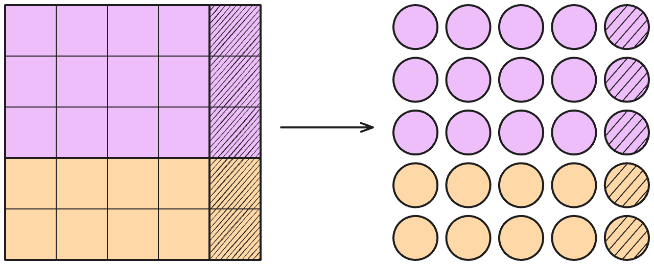
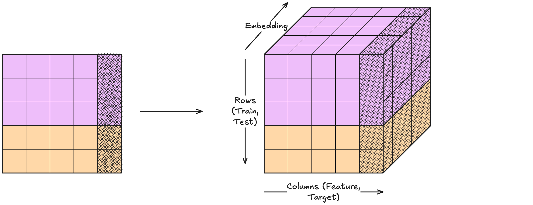
However, representing a table cell with only a single number would be very restrictive. That would be like preparing a complicated dish within one pot. You’d have to do all the cutting, cleaning, frying, boiling all within that pot, no second pot, no cutting board, just the pot. Such an undertaking becomes much easier if you have more processing space. To let tabular foundation models cook, they need some processing space: table cells are internally represented by vectors, also called embeddings. In modern TFMs, the length of these embedding vectors (=embedding size) is larger than in Figure 3.4, for example, 128 for TabPFN-3.0. All table cells are represented by vectors, be it training, test, feature or target.
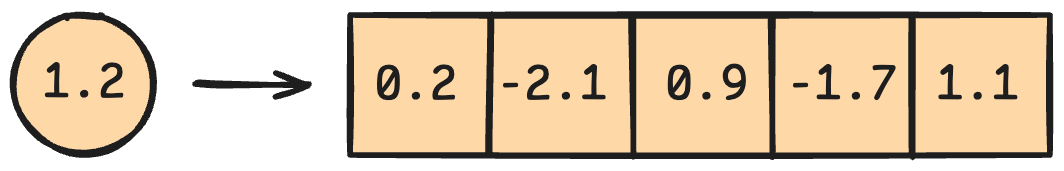
Neural networks typically work with Tensors, and tabular foundation models are no exception. By representing table cells as vectors, we basically blow up the flat 2D table to a 3D tensor, as in Figure 3.4.
While nanoTabPFN has a 1-to-1 equivalent between input table cell and internal representation, most modern TFMs deviate from that. For example, some architectures group features to reduce the number of columns, or introduce new columns to enable more flexible computations.
Embed, transform, decode
Alright, the input is the full table, in between it’s a 3D tensor, and somehow we must end up with a vector or matrix containing the predictions. Time to talk about what happens inside a TFM. The TFM prediction process consists of three steps (again, simplified, mostly applicable to nanoTabPFN with modern TFMs deviating):
- Embed: In this step, the TFM inflates the 2D table to a 3D Tensor. This happens by multiplying a weight vector with each scalar in each table cell and adding a bias. Before that, the features are normalized and clipped. The test targets are pre-filled with the mean target of the training data.
- Transform: Sequentially enrich the information for each table cell by attending to other cells and refining the embeddings. Layer-wise, a “transformation block” includes attention layers, fully-connected layers, norm layers, and skip connections. Multiple transformation blocks are used sequentially.
- Decode: After all the transformation steps, take the embeddings for the test targets and project them back to 2D to make predictions. This is realized through a small, fully-connected network. Decoding is different for regression and classification.
Short: Inflate, transform, deflate (Figure 3.6).
Transform table cells by attending and refining
The transform step is where the heavy lifting happens. A single transform step (for nanoTabPFN) looks like in Figure 3.7. This step is applied a couple of times in a row, e.g. 3 times for nanoTabPFN, and 12 times for TabPFN v2. No need to understand the transformer layer in detail just yet, the main thing we need to form an intuitive understanding: Each transformer layer step enriches the embeddings of the cells, with the main computations being attention and refinement (MLP). Since this transformer layer is repeated multiple times, we may view the “transform” step as an iterative enrichment of the embeddings.
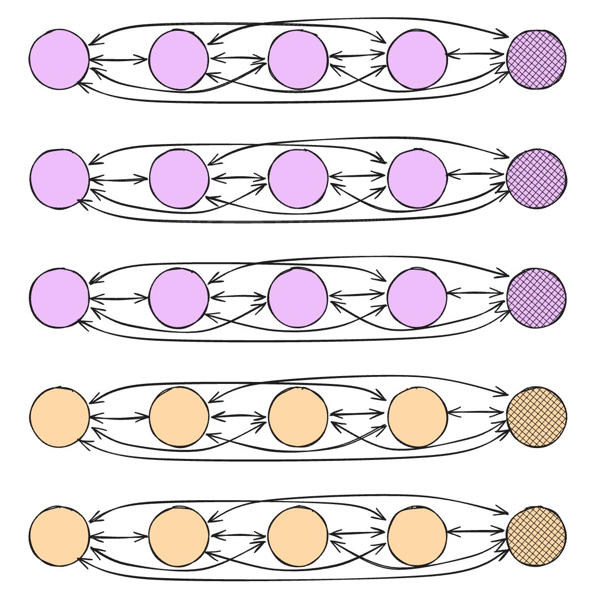
Let’s talk about the attention step first. Attention basically works like a soft lookup table: For example, the model may look up information from other cells to enrich the embedding for Bob’s cholesterol. More technically, the TFM produces a query based on Bob’s cholesterol and it produces keys for each attendable cell. With the query-key match, the TFM weights how much of each attended cell’s values flow into Bob’s updated cholesterol embedding. This lookup is based on the attention-mechanism from the transformer architecture, which we will cover in-depth in the architecture chapter.
Attention has an important restriction: A cell may either attend to all other cells from the same row (e.g., Bob’s hemoglobin level), or the training cells from the same column (e.g., Ari’s cholesterol level), as visualized in Figure 3.8. A restriction for column-attention is that test cells are not attendable, which means both training and test cells may only attend to training data cells.
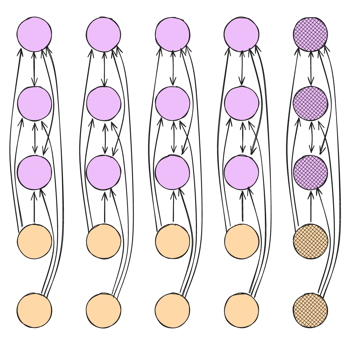
The refinement step takes in only the embedding of a table cell and computes a new representation. Technically, this is realized through two fully-connected layers with non-linear activations, also called a multi-layer perceptron (MLP). This allows the TFM to non-linearly recombine information in the embedding vector. Compute new “embedding features” – with that I mean abstract representation of the embedding, not the table features.
All of these steps from encoding, transforming via attention and refinement, and decoding are based on weight vectors. Weight vectors that have to come from somewhere. This mystical somewhere is the pretraining phase, typically done by the model developers, not by the person applying the TFMs to make predictions. In the next chapter, we talk about the intuition behind pretraining.
I’m talking about test data, but the same applies when making predictions with new data.↩︎