4 Pretraining

By the end of this chapter, you’ll understand that:

TFMs like TabPFN are pretrained, not trained
Pretraining happens on millions of synthetic tasks
The tasks are generated by structural causal models

In this chapter, we explore how tabular foundation models like TabPFN and TabICL are pretrained, which enables the in-context learning we discussed in Chapter 3. Pretraining differs between tabular foundation models, so this chapter focuses on the intuition behind pretraining and what most TFMs have in common (at least the PFN-based ones).

Pretraining instead of training

TFMs have no classic training step. Instead, you provide training data as context at inference time. Technically, the goal of pretraining is to parameterize the millions of weights within the tabular foundation model, which enables it to later do in-context learning.

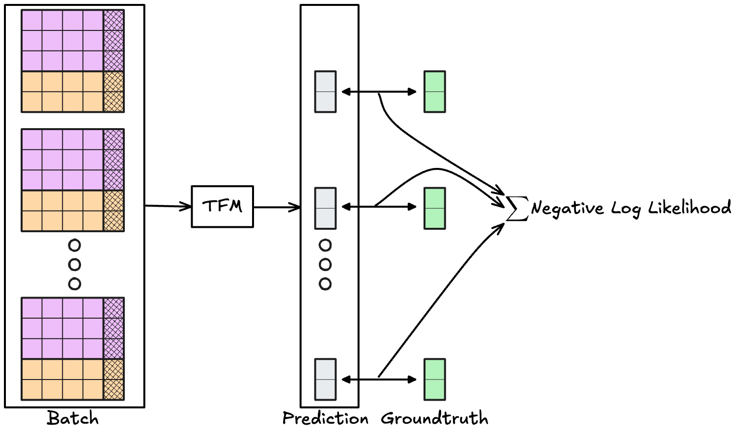
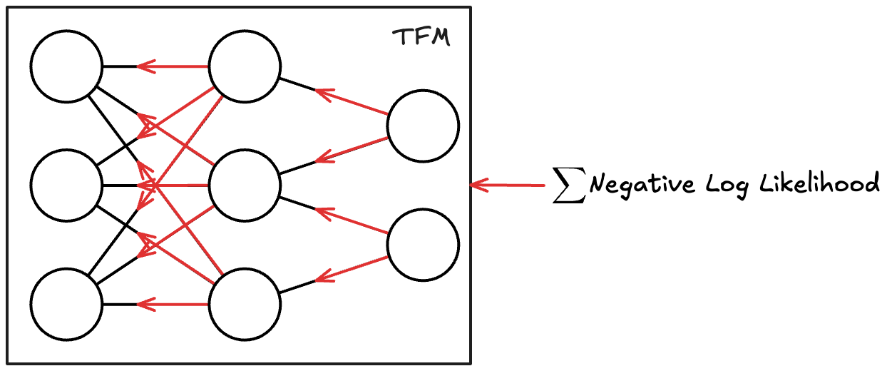
We start with the randomly initialized, transformer-based neural network: Our untrained tabular foundation model. This model is now pretrained on batches of tasks to minimize the negative log likelihood of the prediction of the test targets for each of the tasks. How pretraining differs from tabular training: One “data point” is an entire task and not just a single row of one task. If you can accept this, then pretraining is just stochastic gradient descent via backpropagation updating the weights of the TFM based on how well it solved the batch of tasks. During this pretraining, batches of typically 64 tasks are sent to the model, and the negative log-likelihood is backpropagated to update the model weights. This happens with millions of tasks. Once pretrained, the model is ready to predict without any further, task-specific training, using in-context learning. To get a feeling for just how many datasets a typical tabular foundation model is trained on: TabPFN v2 was trained on 2 million batches of roughly 64 tables, which comes out to around 130 million tables.

Let’s go a bit deeper on the optimization criterion.

Optimizing the negative log likelihood

First, we’ll ignore where the tasks come from – assume we have some machine that gives us infinitely many – and focus on what is being optimized during pretraining. When training a machine learning model, you need feedback on how well the model does, so that you can adapt the weights, grow some trees, or define support vectors. More specifically, for neural networks you need feedback on individual data points or at least on batches of data points. Tabular foundation models are no different, only that the “data points” are entire tasks instead of just table rows. But otherwise, you simply backpropagate the errors the model makes per task, accumulated across the batch, to update the internal weights of the neural network. This is measured with the negative log-likelihood, also called cross-entropy. Simplified, minimizing the negative log-likelihood optimizes the model to predict probabilities for categories. So it’s about making the observed data (the targets) as likely as possible.

To judge how well the tabular foundation model performed for one row in one task, we can compute the negative log-likelihood for this row: \(- \log q_{\theta}(y_{test}|X_{test}, X_{train}, y_{train})\), where \(q_{\theta}(y_{test}|X_{test}, X_{train}, y_{train})\) is the probability output for the correct class (which we know in pretraining). The larger the model’s predicted probability for the correct class, the smaller the negative log likelihood (which can be between 0 and infinite). Add this up for all the test rows in that task, and we know how well the model solved the task. Further add up these sums across all the tasks in the batches, and we have our signal to backpropagate for stochastic gradient descent, see also Figure 4.1 (a) and Figure 4.1 (b).

\[ \mathcal{L}(\theta) = -\sum_{b=1}^{B} \sum_{i=1}^{n_{test}^{(b)}} \log q_{\theta}\!\left(y_{test}^{(b,i)} \mid x_{test}^{(b,i)}, D_{train}^{(b)}\right), \]

with \(B\) being the number of tasks per batch (e.g., batch size 64), and \(n_{test}^{(b)}\) the size of the test data of batch \(b\).

(a) For pretraining, tasks are sent batch-wise (typical batch size is 64) to the TFM. Predictions are scored with the negative log-likelihood.

With the negative log likelihood we have covered the objective for classification, but what about regression? Foundation models for classification and regression are typically pretrained separately, with a different neural network head, and different pretraining tasks. However, a foundation model for regression can still be pretrained with the negative log likelihood, with a binning trick: standardize and bin the target, then treat it like a classification task. This trick is used by TabPFN, which bins regression targets into 999 bins which are treated as categories. Another variant is using a different loss function altogether, like the pinball loss for quantile regression and predicting 100s of quantiles. This approach is used by TabICLv2.

Defining a prior task distribution

Most neural networks need millions of (pre)training data to shine. TFMs are no different, they need lots of tasks. Millions, actually. Ideally, based on diverse datasets. While the (business) world is awash with tabular data, it’s surprisingly hard to get even just hundreds of high quality datasets online.

Fortunately, tabular foundation models can actually be pretrained with synthetic (!) data. Which I still find remarkable, and surprising. I’ll be honest, learning about using synthetic data for tabular foundation models, and seeing them work, completely changed my view on synthetic data. The idea is to design a process that can generate an infinite number of tasks from which we can sample tables.

This task-generating process is called the prior, which comes from the Bayesian framing of pretraining and in-context learning, as covered in Chapter 2. The main “engine” of this task-generating process is the structural causal model (SCM), which tells us for a bunch of variables how they are related to each other.

There are 3 different levels of abstraction involved in the process to generate the synthetic pretraining data, also visualized in Figure 4.2:

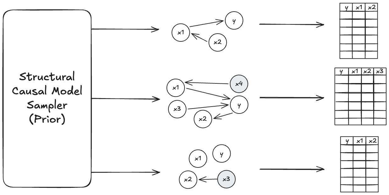
Figure 4.2: To generate data for pretraining, sample structural causal models from the prior, and sample one dataset from each structural causal model.

First, we need a generator for structural causal models. This includes sampling mechanisms for high-level parameters such as number of variables in the SCM, but also a recipe for generating them.
From this generator, we can sample an infinite amount of SCMs. Each SCM describes the relationships of a bunch of variables, such as the number of variables, and how they are related to each other.
To get a dataset, we can generate data rows from the SCM. We sample a subset of the variables and designate one as the target.

But what is a structural causal model and why is it so useful for pretraining tabular foundation models?

Synthesizing a structural causal model

Structural causal models, or SCMs for short, describe causal relationships between variables. You can visualize an SCM partially as a directed acyclic graph (DAG), as in Figure 4.3:

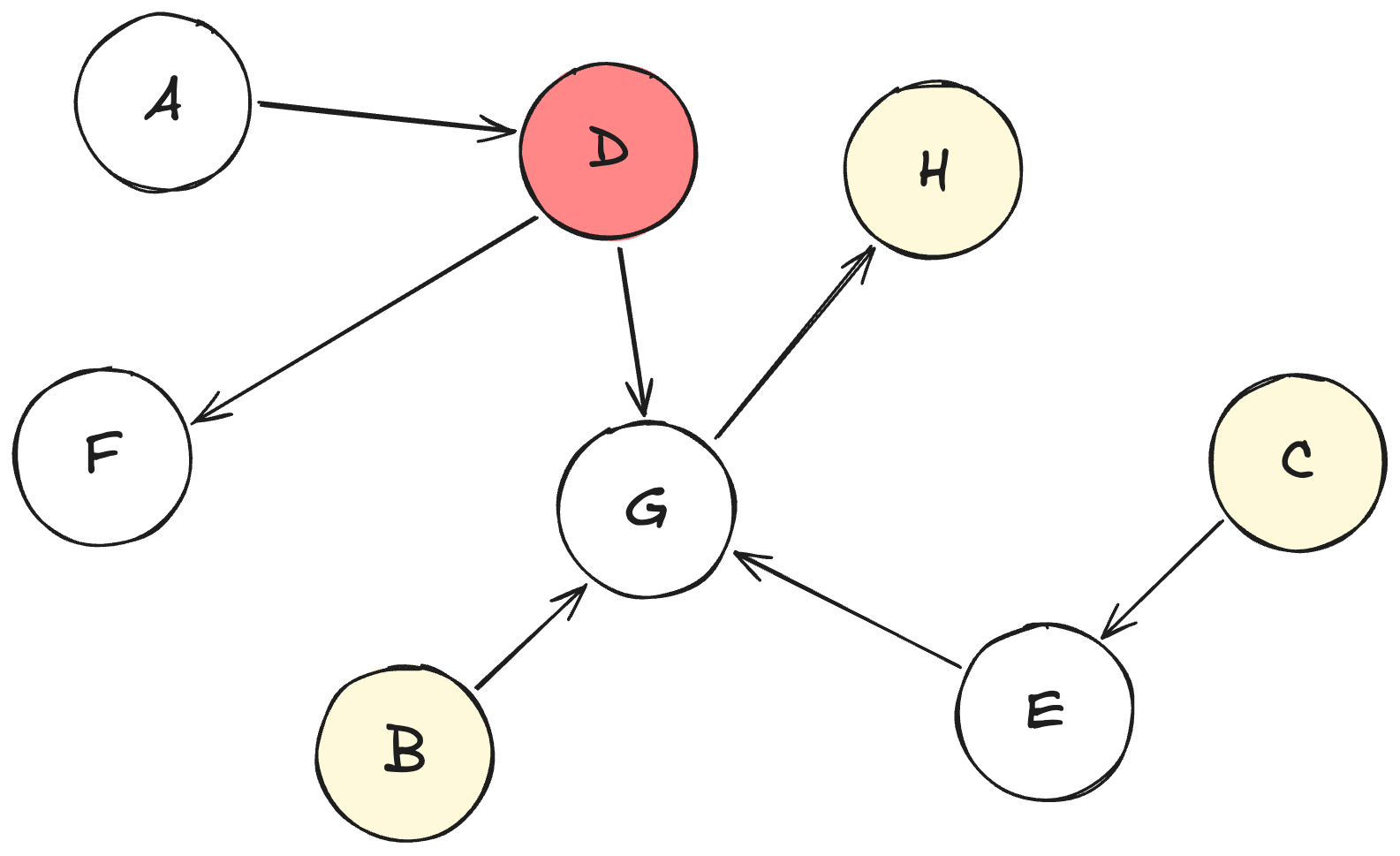
Figure 4.3: Example of a directed acyclic graph.

Let’s interpret this DAG:

Each node from A to H is a variable.
Each arrow indicates a causal relationship, for example, variable A causes variable D.
We call some nodes parents and some child nodes: For example, D is a child node of A, which makes A a parent for D. D itself is also a parent node to F and G.
Variables will later have different (sampled) roles:
- D is the target
- B, C, and H are the features
- A, E, F, G won’t make it into the data (“unobserved”)

The visualization as a directed acyclic graph does not contain all the information of an SCM, we further have:

All the functions that describe how a child variable depends on the parent nodes. For example, variable G might be a linear function of B, D, and E, and E might be sign(C).
The SCM also describes the error terms that additionally influence a variable. For example, variable “G” might be a linear combination of B, D, and E plus some error term.

For pretraining, these SCMs are randomly generated. The random generation involves high-level parameters such as the number of variables, the connectivity, the randomly assigned dependency functions, and so on. However, we won’t go into the details and intricacies of SCM sampling. In addition, one needs a construction algorithm that ensures that the graph stays directed and doesn’t become cyclical.

What’s so special about structural causal models? As the name implies, SCMs reflect causal structures: Some variables influence the value of another variable, plus some sources of randomness. Developers of TFMs now mostly use structural causal models to generate pretraining data. A pretty interesting fact. It shows that the SCMs are tremendously effective in helping tabular foundation models predict real world data. This is speculative, but I interpret this as SCMs being actually a good emulation of underlying structures of the real world, or at least their representations in data.

Next up, we need to sample a dataset from an SCM.

Sampling a task from a structural causal model

The SCM is just a stepping stone. What we actually want is a task, which includes a table, a feature-target indicator, and train-test indicators. This means we have to generate a dataset from an SCM. Here is a high-level summary of how to sample a row from an SCM (we can apply this in parallel for all rows):

Start with variables without parents: Sample their values, typically from Gaussian or uniform noise. In Figure 4.3, this would be nodes: A, B, C.
Forward-propagate values through the graph, based on the relationships described by the arrows. Thereby, the cell value for a child is based on the values of the parents, the function describing the relationship, and the error function.
- For Figure 4.3, after the initial step, we would continue with D as a function of A and E as a function of C.
- Next would be G as a function of E, B, and D.
- Last is H as a function of G.

We are not done yet, as we have to turn the table of variables into a task of features and targets.

Sample which of the variables are targets, features, or remain unobserved.
Throw away the unobserved variables.
Take all the variables that are marked as features or targets and create a table from them. Mark some of the rows as training data and the others as test data.

Like this, on the fly, you can sample SCMs from the prior, and for each SCM, sample one dataset. 64 datasets create a batch. Pretrain the model a bit more. Repeat with more batches until convergence or your GPU credits run out, or someone else needs the GPU cluster.

The prior is of utmost importance

Clearly, the prior is essential: without it, there is no foundation model. However, besides wanting to have a prior with a great volume of datasets, we want it to represent a diverse set of tasks: Tasks with different numbers of features, from just one feature to thousands or millions. Tasks with complex non-linear relations; but also tasks with only noise features. Tasks with many important non-observed variables; tasks where we observed all relevant variables. I could continue this list, but the essence is that pretraining should cover a broad range of scenarios. Adding tasks with specific characteristics instills inductive biases into the foundation model.

Definition: Inductive Bias

Preference of an algorithm to prefer one pattern over another.

So we can see the prior as a catalogue of task characteristics. By adding to that catalogue, we can “upgrade capabilities” of the tabular foundation model. Here are just a few examples:

Tree-based biases: TabICL (Qu et al. 2025) adds SCMs with tree-based functions for relations between variables into the prior (30% of tasks). This instills inductive biases of tree-based models directly into pretraining.
High-frequency oscillations: TabPFN-3 (Prior Labs Team 2026) adds sinusoidal activations to the prior, which improves performance on datasets which exhibit frequency data (oscillations).
Extrapolation: TabPFN-3 (Prior Labs Team 2026) adds out-of-distribution prediction tasks to its prior, which helps the model with extrapolation, meaning to predict outside the range of the feature support.